Worked Example 5 - Combined Trial Modelling • vectorpower

In the previous worked example, the use of the cohort() function to simulate the cluster cohorts in the control and intervention arms of a field trial after setting up the clusters using the cluster_input_setup() and clusters_create() function (as described in example 3 was demonstrated. This process can be simplified by using the crt_combined() function as described in the example below.

As before, first load the package (install it first if necessary as shown in the Installation article:

library(vectorpower)

As in previous examples, the main population data set is loaded from an RDS file created by saving the results of running the mainpop() function (see Worked Example 2).

# Load main population data
mainpop_data <- readRDS(file=url("https://github.com/KeithJF82/vectorpower/raw/master/inst/extdata/DemoFolder1/mainpop_data.Rds"))

[Note on displaying year-round data TBA]

data_view1=data.frame(n=mainpop_data$annual_data$n_mv,EIR_annual=mainpop_data$annual_data$EIRy)
matplot(x=data_view1$n,y=data_view1$EIR_annual,type="p",pch=1,xlab="Dataset",ylab="Annual EIR")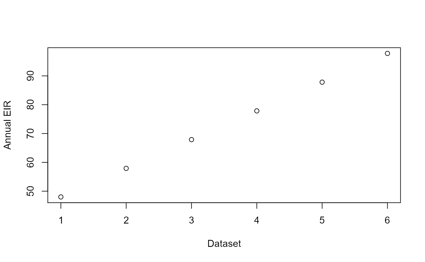

[Note on displaying mainpop results TBA]

data_view2=get_mainpop_data(input_list=mainpop_data,benchmark="EIR",set_n_mv=mainpop_data$n_mv_set)
plot_mainpop_data(data_view2)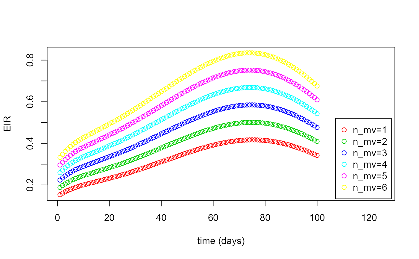

The crt_combined() function takes in inputs for the cluster_input_setup(), clusters_create() and cohort() functions and runs them for the control and intervention arms

test_time_values=10.0*c(1:10) # Time points at which testing takes place
n_clusters=10             # Number of clusters to generate
benchmark="EIR_annual"    # Main population data parameter to use as benchmark for generating clusters
benchmark_mean=75.0      # Mean value of benchmark to use to create distribution
benchmark_stdev=5.0     # Standard deviation of benchmark to use to create distribution
int_mean=0.1              # Mean value of intervention parameter (ATSB mortality rate) in intervention clusters
int_stdev=0.0             # Standard deviation of intervention parameter in intervention clusters
prop_T_c = 0.9            # Proportion of clinical cases receiving treatment independent of trial-related testing
n_patients=100            # Number of patients per cluster
age_start=0.5             # Minimum age of cohort patients
age_end=10.0              # Maximum age of cohort patients
test_type="RDT"           # Type of test administered to  patients ("clin" = clinical, "RDT" = rapid diagnostic test)
flag_pre_clearing=1       # Integer indicating whether patients given pre-trial prophylaxis (if 1, place all patients                               into prophylaxis category at start)
censor_period=10.0         # Time period after a positive test during which a patient is not counted towards incidence
flag_reactive_treatment=1 # Integer indicating whether patients are automatically given prophylaxis after a positive                                test (shifting them into treatment category if a clinical case, prophylaxis category                                    otherwise)
flag_output=0             # Integer indicating whether to show progress of simulation
data_level="Both"         # Data type to output ("Cluster", "Individual" or "Both")
output <-
crt_combined(mainpop_data=mainpop_data,n_clusters=n_clusters,n_patients=n_patients,benchmark=benchmark,
             age_start=age_start,age_end=age_end,test_time_values=test_time_values,test_type=test_type,
             flag_pre_clearing=flag_pre_clearing,censor_period=censor_period,
             flag_reactive_treatment=flag_reactive_treatment,prop_T_c=prop_T_c,
             benchmark_mean=benchmark_mean,benchmark_stdev=benchmark_stdev,int_mean=int_mean,int_stdev=int_stdev)
#> 
#> Simulating control clusters
#> Simulating intervention clusters
#> Outputting control cluster data (cluster level)
#> Outputting intervention cluster data (cluster level)
#> Outputting control and intervention cluster data (individual level)

[Text about viewing output data]

head(output$output_indiv)
#>   Date Patient Cluster Trt      Age Het_cat Status Test_status het_cat
#> 1   10       1       1   0 2.666667       0      0           0       4
#> 2   20       1       1   0 2.666667       0      1           1       4
#> 3   30       1       1   0 2.666667       0      0           0       4
#> 4   40       1       1   0 2.666667       0      0           0       4
#> 5   50       1       1   0 2.666667       0      0           0       4
#> 6   60       1       1   0 2.666667       0      5           0       4

[Text]

control_plot <- plot_cohort_data(cohort_data = output$cohort_data_con,benchmark = "test_inc",flag_output=2)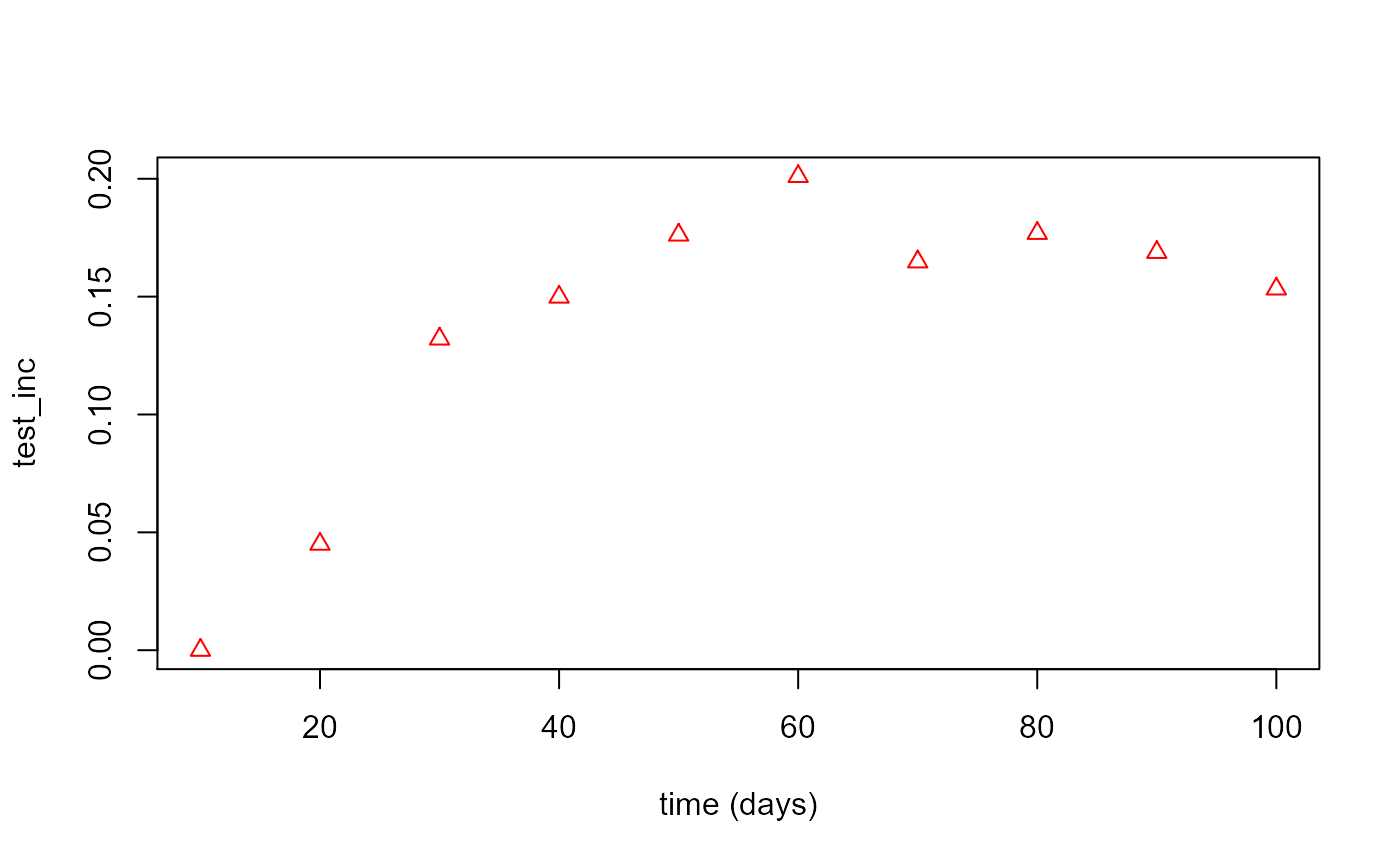

int_plot <- plot_cohort_data(cohort_data = output$cohort_data_int,benchmark = "test_inc",flag_output=2)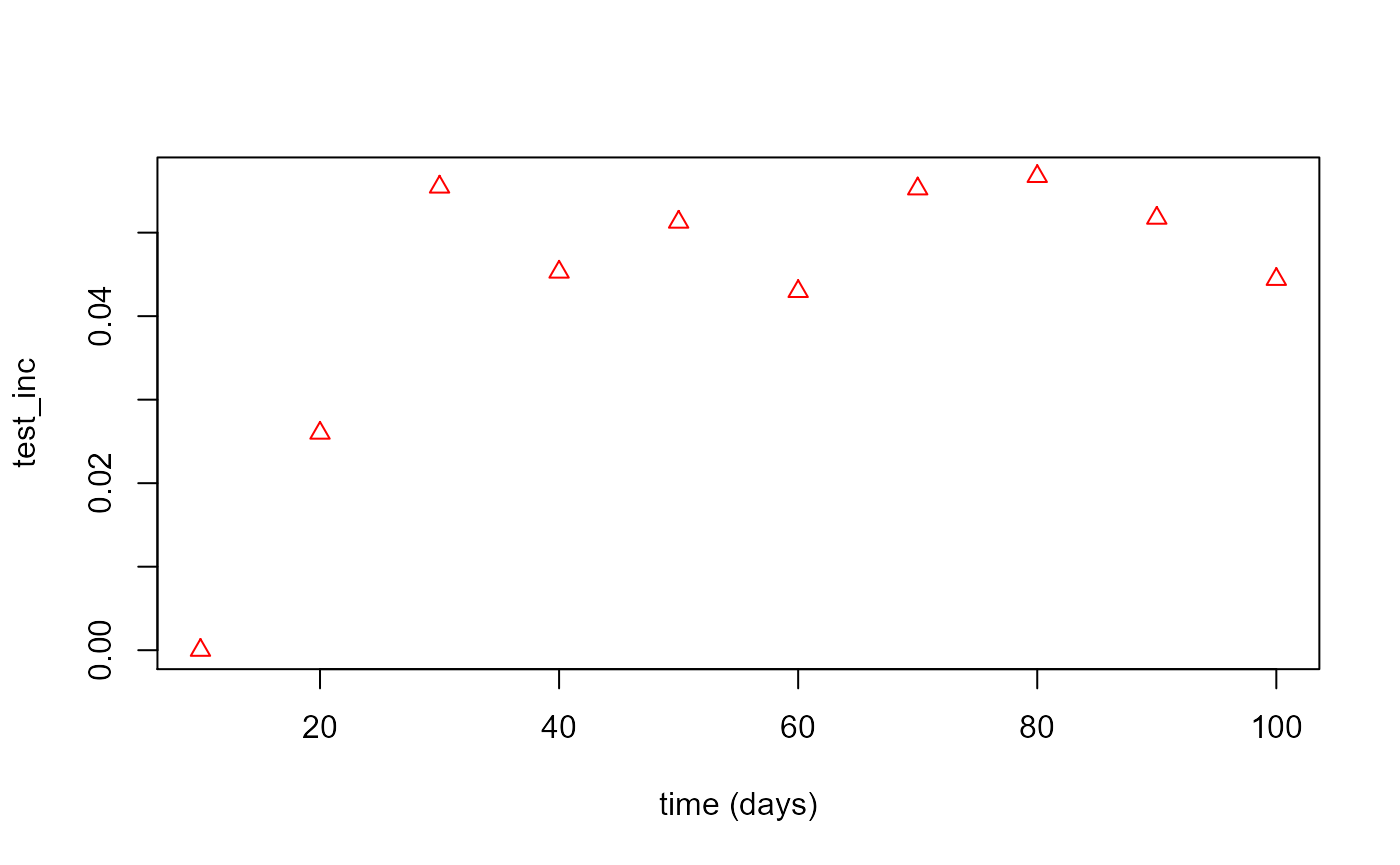

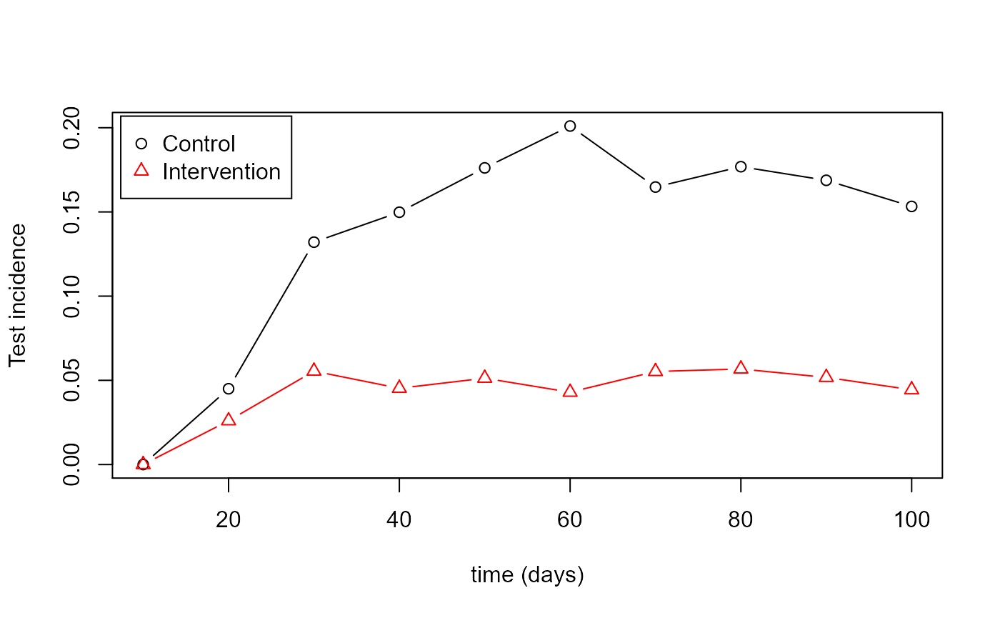
matplot(test_time_values,control_plot,type="b",pch=1,lty=1,col=1,xlab="time (days)",ylab="Test incidence"
        ,ylim=c(0,max(control_plot)))
matplot(test_time_values,int_plot,type="b",pch=2,lty=1,col=2,add=TRUE)
legend("topleft", inset=0.01, legend=c("Control","Intervention"), pch=c(1:2),col=c(1:2),
       horiz=FALSE,bg='white',cex=1.0)