Introduction

This document introduces the vectorpower package It is based on the content of the associated poster presented at the ASTMH Annual Meeting in November 2019 and the associated handout. A PDF copy of this poster can be found at https://tinyurl.com/rlkojta. For further information, please contact keith.fraser@imperial.ac.uk.

The vectorpower package is designed to facilitate the simulation of cluster randomized trials (CRTs) of vector control interventions against Plasmodium Falciparum malaria. The interventions currently included are long-lasting insecticide-treated nets (LLINs), interior residual spraying (IRS) and attractive targeted sugar baits (ATSBs). Potential applications include:

Estimating population-wide effects of vector control interventions
Predicting potential observed cohort data in control and intervention clusters in CRTs
Estimating statistical power of CRT designs
Informing future CRT design

Software

The package is created in the R language. It uses the C++ language for the actual simulation of malaria progression in humans and mosquitoes, using an existing numerical malaria model (J.T. Griffin et al, Lancet Infect Dis. 16 465, 2016). The current version of the package can be found at https://github.com/KeithJF82/vectorpower. It is still being added to with new features and documentation; feedback from users and potential users is welcomed.

It is intended for users to be able to carry out all the steps involved in simulating a CRT starting from basic parameters, as shown in Fig. 1. Some steps may be omitted depending on desired outcome and available data, e.g. a user may use saved initial state or main population data for a new simulation to save time.

Fig. 1

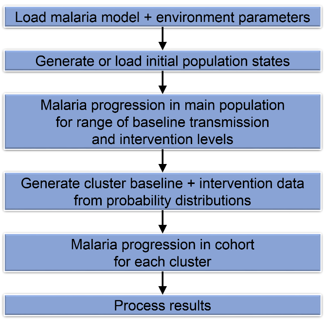
The parameter values required by the malaria model are stored as files and can be adjusted manually. The environmental parameters include those used to calculate rainfall (which controls mosquito larval hatching rates) as a function of time of year, and any pre-existing intervention levels.

Initial population state data is created by calculating values at steady state (constant rainfall), then simulating malaria progression over several years under variable rainfall conditions to reach equilibrium. This is carried out for multiple baseline malaria levels based on user input.

The user specifies a subset of the initial state data to use, along with a range of values of the varied intervention parameter (coverage of LLINs or IRS, or additional death rate due to ATSBs). Simulation of the mosquito population and main human population (the set of all humans in a group, as opposed to the trial cohort) is then carried out for all parameter combinations over the trial period. These populations are simulated using a deterministic continuum model.

The main population simulation data is then used as a group from which to draw individual clusters. Normal cumulative probability distributions are created by setting mean and standard deviation values of the varied intervention parameter and one of various malaria benchmarks (prevalence, incidence or entomological inoculation rate at a particular time in the main population simulation, or the annual EIR at equilibrium). A number of clusters are then generated from these distributions, each associated with a set of data from the main population simulation.

The trial cohort in each cluster is then simulated using a stochastic individual model, with EIR and starting immunity data taken from the output of the main population calculations. The results represent the data that will be gathered in a CRT.

Example

This section describes a typical example of how the package may be used to simulate the results of a CRT. The example used is an ATSB epidemiological trial, to be carried out from July-December in an area with highly seasonal malaria where the year-round EIR has a mean value of 100 infectious bites/person and a standard deviation of 20. The additional death rate due to ATSBs is expected to vary between 0.0 and 0.2/day.

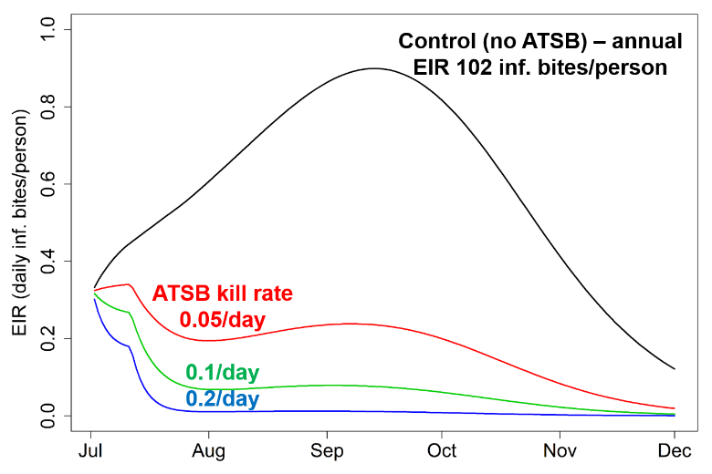
Initial state data consists of 31 sets of values representing year-round annual EIR values ranging from 37.9 to 198.3 infectious bites/person. The intervention parameter (ATSB killing rate) is varied in the specified range over 41 points. When the mosquito and main human populations are simulated over the trial period, 1,271 sets of values are therefore produced. (This requires several hours’ computation time on a typical desktop PC.) Fig. 2 shows how daily EIR varies over time for different intervention parameter values for a particular set of initial data.

Fig. 2

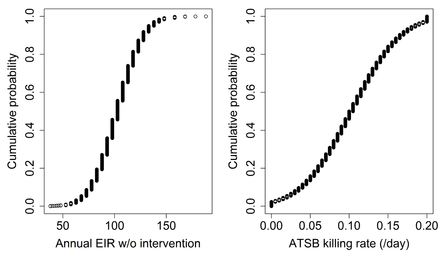
The mean and standard deviation of the EIR given above are used to generate a cumulative probability distribution (Fig. 3A) from which to generate clusters. The intervention parameter distribution (Fig. 3B) is based on a mean ATSB killing rate of 0.1/day with a standard deviation of 0.05/day, producing a truncated distribution due to the permitted values being confined to the range used in simulations.

Fig. 3

Two sets of clusters representing possible outcomes in the control and intervention arms of the trial are then produced. The control clusters are generated using a mean and standard deviation of 0 for the intervention parameter, so that only data for an ATSB killing rate of 0 is used. The intervention clusters are generated using both distributions, allowing them to be drawn from all 1271 sets of results. This gives each cluster an associated set of daily EIR values like those in Fig. 2, as well as starting patient immunity parameter values.

The trial cohorts in 10,000 clusters of each type are simulated over the trial period to produce a distribution of outcomes. (This along with the generation of the cluster data requires only a few minutes’ computation time, allowing many different scenarios to be quickly explored using the same main population data.) 100 patients between the ages of 6 months and 10 years are simulated per cluster, and are initially assumed to be malaria-free. Fig. 4 shows how the average malaria prevalence in the cohort measured monthly over the trial period varies across the sets of clusters. Other values output by the simulations can be used as the outcome, such as final prevalence, total incidence over the trial period, etc.

Fig. 4

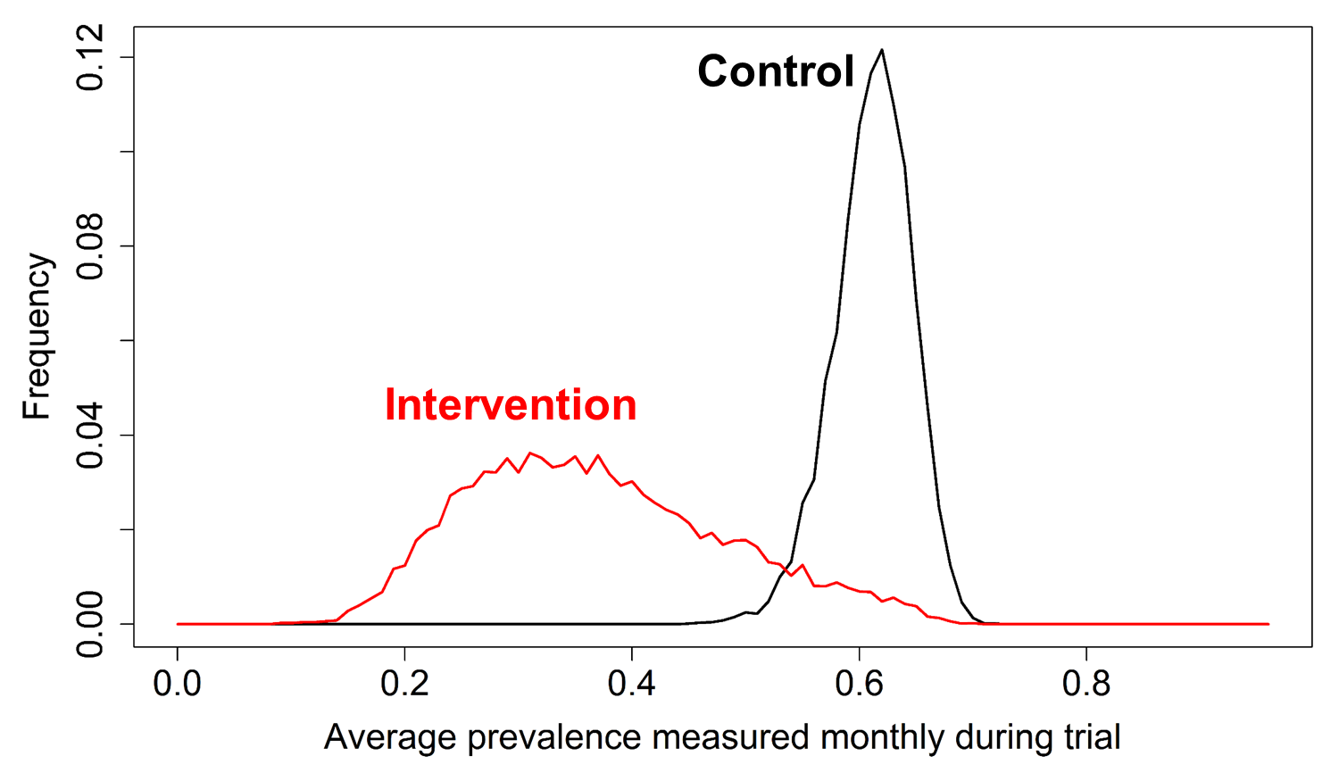
As shown in Fig. 4, the average prevalence measured during the trial in an intervention cluster will generally be significantly lower than that measured in a control cluster, but not 100% of the time due to the overlap between the outcome frequency distributions. The probability β of a type II error (null hypothesis erroneously not rejected) can be estimated by repeatedly comparing one or more random clusters of each type.

A trial with only one control and one intervention cluster is used with the null hypothesis that the intervention cluster will show less than a 30% drop in average prevalence compared to the control cluster. For 10,000 repetitions, β=0.295, giving a statistical power (1-β) of 70.5%. If the trial is expanded to include 2 control and 2 intervention clusters, with the prevalence values in each pair being added together, the estimated power with the same null hypothesis rises to 76.8%. Other trial design options can also be explored using the package, such as varying the number of patients in each cluster cohort.